Published in: The IEEE Control Systems Letters (L-CSS)
Authors: Seungjoon Lee and Hyungbo Shim
DOI: 10.1109/LCSYS.2019.2916250
Abstract: Economic dispatch problem for a networked power system has been considered. The objective is to minimize the total generation cost while meeting the overall supply-demand balance and generation capacity. In particular, a more practical scenario has been studied by considering the power losses. A non-convex optimization problem has been formulated where the non-convexity comes from the nonlinear equality constraint representing the supply-demand balance with the power losses. It is shown that the optimization problem can be solved using convex relaxation and dual decomposition. A simple distributed algorithm is proposed to solve the optimization problem. Specifically, the proposed algorithm does not require any initialization process and hence robust to various changes in operating condition. In addition, the behavior of the proposed algorithm is analyzed when the problem is infeasible.

This work is a continued effort of CDSL to tackle the distributed optimization problem and its application to the economic dispatch problem (EDP). For our previous works, see https://post.cdsl.kr/archives/1263 or https://post.cdsl.kr/archives/615. This post only sketch the main ideas of the paper. For more technical details, refer to the paper.

What is the Economic Dispatch Problem?

The economic dispatch problem (a.k.a. resource allocation problem) is a fundamental problem which arises in the operation of the power network. The EDP considers a network of $N$ nodes, each with power demand and supply. The main objective is to balance the overall power supply and demand. At the same time, we would like to respect various additional constraints such as local general constraint and minimize overall generation cost. The following illustration gives a common scenario for the EDP.

A common scenario considered in the EDP.

Economic dispatch problem is often formulated into an optimization problem (which we call original problem) given by

where $f_i(x_i)$ are strictly convex cost functions, $\mathcal{X}_i$ denotes the local generation constraints and $\sum d_i = \sum x_i - \phi(x)$ denotes the global supply and demand balance and $\phi(x)$ is a nonlinear function which models the losses.

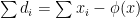
Most of the existing literature on EDP solve the problem formulated as above with $\phi(x) = 0$ ., i.e., there are no losses. Unfortunately, in practice, generation and transmission of power always come with various forms of losses. Hence, these effects are ignored with such a simple formulation. However, solving the EDP considering the loss is particularly important as various losses can be up to 10% of the generation.

In this work, we suppose that the losses of the system $\phi(x)$ is a separable function, i.e., it can be written as

$$\phi(x) = \sum_{i=1}^N \phi_i(x_i)$$

where $\phi_i(x_i)$ is the loss of the node $i$ . Separable loss function can represent simple models for the transmission losses, as well as the generation loss of each generator.

Challenge when dealing with losses

As this work consider the losses of the system, this leads to two main challenges compared with previous works.

1. Nonconvexity of the Problem

Note that the formulated optimization problem with nonlinear loss function is not a convex optimization problem. Hence, it is in general hard to solve for the optimal solution. In order to overcome this challenge, we relax the original problem into the following

where we have relaxed the nonlinear equality constraint into an inequality constraint. Therefore, the relaxed problem is now convex and can be solved efficiently (in a centralized manner).

However, it should be asked whether the optimal solution obtained from the relaxed problem is at any use. Specifically, there are no reasons to solve the relaxed problem if its results are not meaningful. For this, we make following assumptions.

Monotonic cost function $$ 0 < \frac{df_i}{dx_i}, \quad \forall x_i \in \mathcal{X}_i$$
Realistic Loss Model $$ \frac{d\phi_i}{dx_i} < 1, \quad \forall x_i \in \mathcal{X}_i$$

Both of the assumptions are easily satisfied in case of the EDP. For instance, it is typical to use a quadratic cost function given by 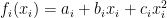$f_i(x_i) = a_i + b_ix_i + c_ix_i^2$ with $b_i>0, c_i>0$ . In addition, the second assumption states that the incremental loss cannot be larger than the incremental generation, which is reasonable for the physical systems.

Fortunately, under the stated assumptions, it can be shown that the optimal solution obtained from the relaxed problem is in fact also optimal to the original problem. Therefore, we can instead solve the relaxed problem (which is convex) instead of the original problem (which is nonconvex) for the solution.

2. Constrained Dual Problem

Since the relaxed problem is convex, the relaxed problem can be formulated into the dual problem using similar techniques from this result and hence details are not discussed. In conclusion, we can obtain the dual problem for the relaxed problem as stated below.

Here, $g_i$ is the dual functions, $\mathcal{L}_i$ is Lagrangian, $\lambda$ is the dual variable and $\hat{x}_i$ is a static mapping defined as

The function $v_i$ is defined using the local cost function and loss function, and its exact form can be found in the paper.

The main difference with previous results is that now the dual problem is a constrained optimization problem. The constraint $\lambda \geq 0$ comes from the relaxation of the original equality constraint into an inequality constraint. Oftentimes, the constrained optimization problem is solved using projection. However, these are harder to implement in practice due to discontinuous vector fields. Instead, we simply extend the domain of the function $\hat{x}_i$ into $\mathbb{R}$ as

Interestingly, it can be shown that even with the new modified dual function, the dual problem is still concave and hence it is a concave, unconstrained optimization problem. Moreover, the vanilla gradient ascent algorithm can be applied to obtain the optimal solution.

Finally, it has been shown in the paper that the solution to the modified dual problem (which can be obtained via vanilla gradient ascent algorithm) is, in fact, an optimal solution to the original problem we wanted to solve.

Distributed Solution

The gradient descent algorithm proposed in previous section is a centralized algorithm. However, it can be easily converted into a distributed algorithm using the concepts of the blended dynamics as below.

$$\dot{\lambda}_i = \frac{d\mathcal{L}_i(\hat{x}_i(\lambda_i),\lambda_i)}{d\lambda_i} + k \sum_{j \in \mathcal{N}_i} (\lambda_j – \lambda_i)$$

where $\lambda_i$ is the estimate of the dual variable. Its blended dynamics is given by

$$\dot{\lambda} = \frac{1}{N} \sum_{i=1}^N \frac{d\mathcal{L}_i(\hat{x}_i(\lambda),\lambda)}{d\lambda}$$

which is the centralized gradient ascent algorithm (with some scaling factor). Hence, using the theory of the blended dynamics developed at CDSL, it holds that the solution of the distributed algorithm approximately converges to the optimal solution.

Further Discussions

The paper contains additional results for the proposed distributed algorithm. For instance, although the algorithm converges approximately, it is shown that the overall supply and demand balance is always satisfied exactly. Moreover, the behavior of the algorithm is also analyzed when the problem is infeasible. If you are interested, please see our paper for these results.

Distributed Algorithm for Economic Dispatch Problem With Separable Losses